Discovery rarely comes from one perfect guess. It advances through repeated rounds of proposing an idea, testing it and learning what to try next. LDM is built for that loop: each result helps it decide which possibility is worth testing next, so fewer costly evaluations are wasted.
The paper tests LDM on three computational benchmarks. In each one, results from an earlier round guide what the system tries next. Here are the final reported comparisons in plain language.
MODEL TRAINING
2.4 times
the reduction in prediction loss
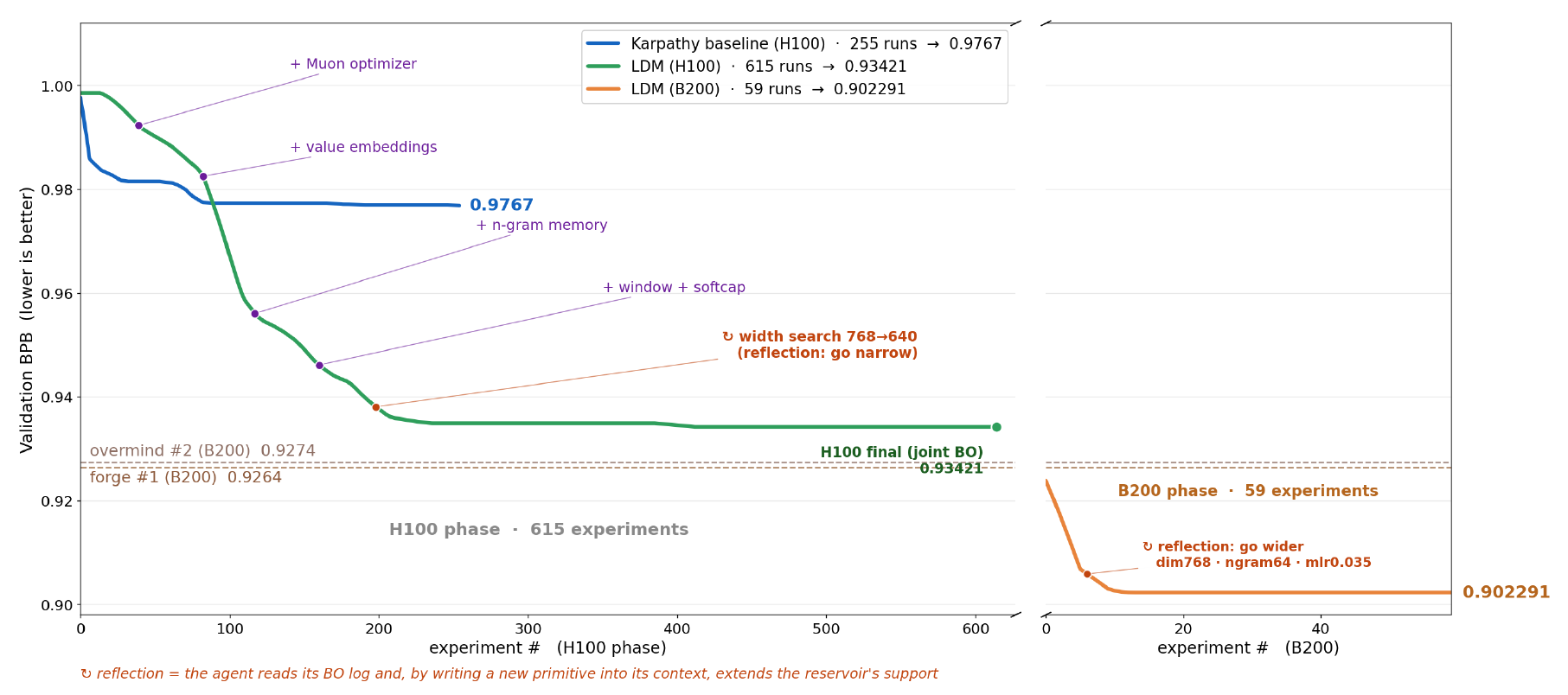
Starting from the same model, LDM reduced prediction loss on unseen text from 1.0069 to 0.9342. The LLM-only Karpathy baseline reached 0.9768.
Lower is better. This compares reductions from the same starting point, not equal numbers of experiments.ANTIBODY DESIGN
18.2 per cent
more favourable computational binding score
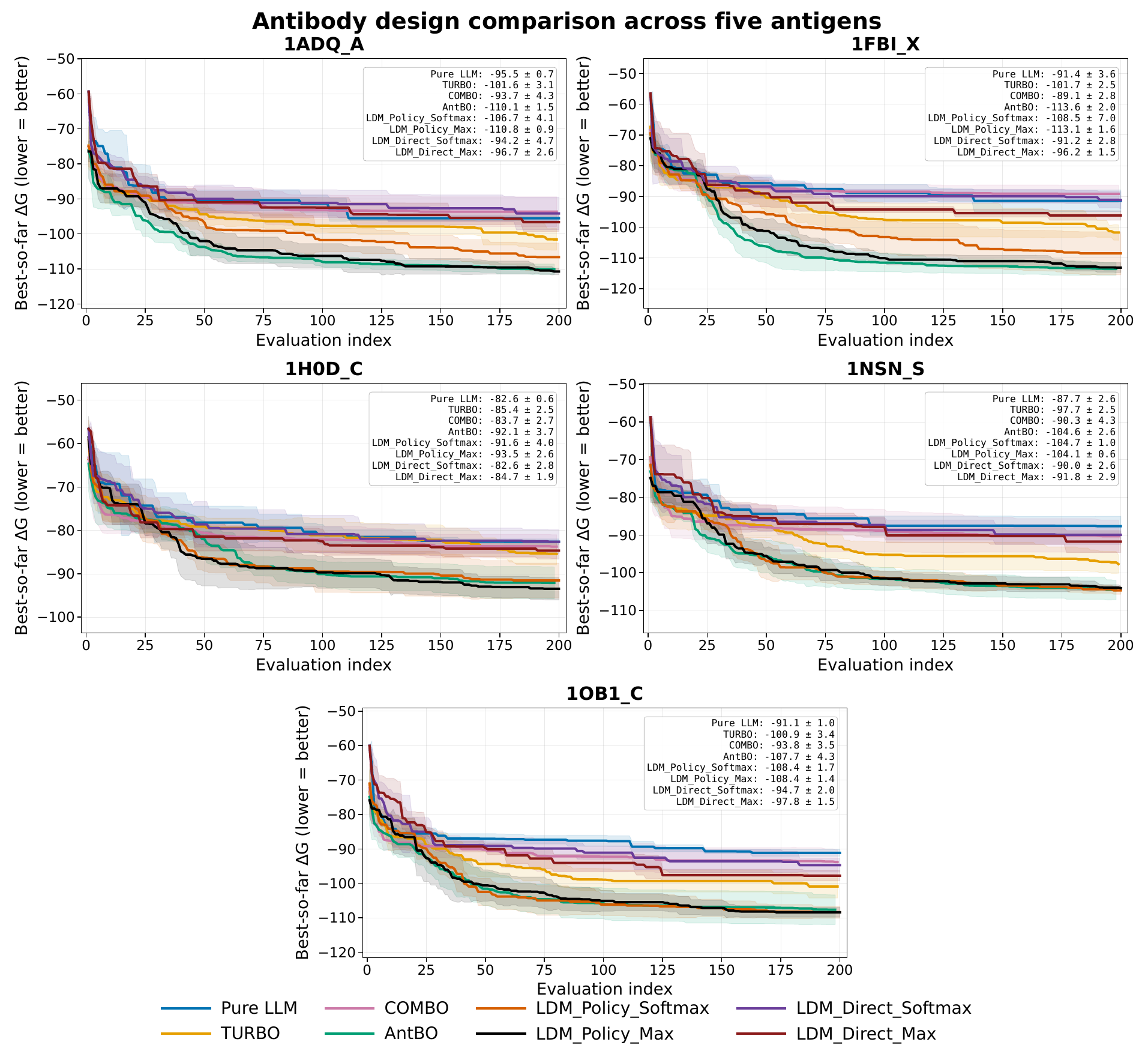
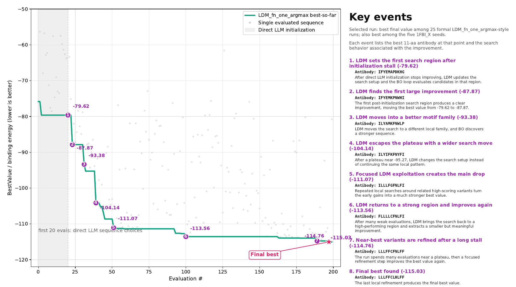
Across five targets, Policy-Max LDM achieved an average score of negative 105.98, compared with negative 89.66 for Pure LLM.
More negative is better in this simulation. These are computational scores, not laboratory measurements.MOLECULE DESIGN
62.4 per cent
higher multi-objective score than Pure LLM
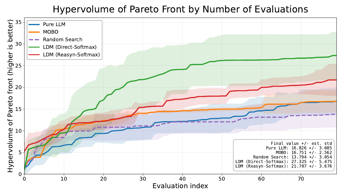
LDM reached 27.325, compared with 16.826 for Pure LLM and 16.751 for multi-objective Bayesian optimisation.
This score rewards strong trade-offs across docking and predicted activity. Higher is better. LDM was 63.1 per cent above MOBO.
These tasks are examples, not the boundary of the method. LDM is designed for any large design space where tests are costly and each result can guide the next round.
How can AI search a space too large to list when every test is expensive?
One reason language models have advanced in mathematics, code, and games is that candidate answers can be difficult to find yet comparatively easy to verify. Programs can be tested, games have explicit rules, and derivations can be checked. A model can generate many candidates, then spend test-time compute comparing and revising them.
Discovery has different economics. A candidate might be a material recipe, an engineering design, an experimental protocol or a software system. Testing it may require specialist equipment, scarce samples, sustained computation or expert review. The design space is open-ended when its candidates cannot be listed in advance and the way they are generated determines which possibilities the system can reach.
The aim is not to guess correctly in one attempt. The system repeats four steps: read what is known, propose possibilities, choose a few to test, and use the results to decide what comes next. A useful system must improve both its ideas and its choice of experiments.
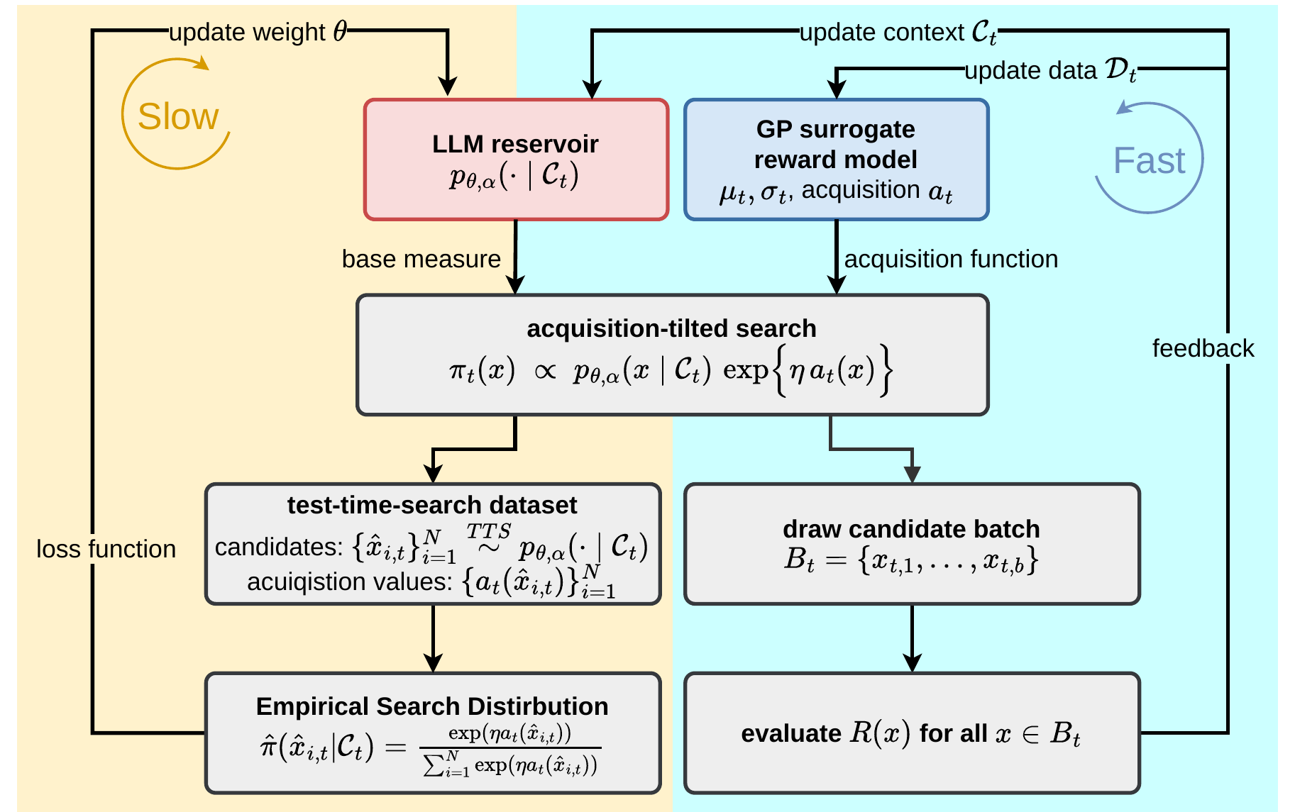
LDM has three components, each with a different job. The LLM proposes possible designs. A lightweight prediction model learns from experiments already completed and estimates which candidates look promising and where the system is still uncertain. A decision rule then chooses which candidate is worth spending the next evaluation on. In the paper, these three components are called the proposal model, surrogate model, and acquisition function.
WHY THIS IS HARD
AI cannot test everything. It has to choose what is worth trying next.
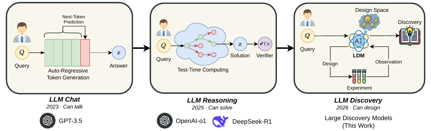
In ordinary dialogue, the model produces an answer and stops. In a reasoning system, it can try multiple candidates and filter them with a cheap, repeatable verifier. Discovery adds another layer of difficulty: feedback comes from an external evaluator and may be expensive, delayed or noisy. The system must decide which few evaluations deserve the available budget.
If every candidate were already listed, the system would only need to rank them. In an open-ended space, the candidate list itself changes during search. The generator determines what the system is able to consider at all. The experimental results then help decide which of those possibilities deserves the next test.
Three different feedback regimes: dialogue produces one response; reasoning compares candidates with a cheap verifier; discovery chooses a small number of interactions with an external evaluator and lets the outcomes change what is proposed next.
LANGUAGE MODEL
It can suggest ideas, but cannot reliably judge them
Language-model likelihood measures whether a proposal resembles patterns in its training data. It is not a reliable estimate of performance under an external objective, and model confidence is not calibrated epistemic uncertainty.
BAYESIAN OPTIMISATION
It can choose only from candidates it has seen
Bayesian optimisation can use sparse results to balance promise and uncertainty. But it cannot select a strong design that the generator never produced.
HOW LDM WORKS
Each test changes what the system tries next.
LDM proposes possibilities, chooses one to test, learns from the result and begins the next round with better evidence.
01
Propose possible designs
The LLM reads the objective, constraints and evidence so far, then suggests possibilities for the next round.
02
Learn from completed tests
A small prediction model uses earlier results to estimate what looks promising and where the system is still uncertain.
03
Choose the next test
A decision rule weighs promise against uncertainty and selects the candidate most worth evaluating next.
04
Use the result in the next round
The new result becomes part of the evidence, changing both how candidates are judged and what the LLM proposes next.
What this figure shows: the fast loop proposes, tests and learns from candidates. The slower loop trains those successful search decisions back into the model, making the strategy cheaper to reuse.
DETAILED RESULTS
The same loop produced gains in three very different tests.
These case studies test the general framework; they do not define its boundaries. Each uses a different kind of design, external test and comparison method.
One framework, tested across three kinds of design space and three different evaluation signals.
Case study
Design space
Evaluation metric
Task scope
Evaluation budget
AutoResearch
Possible changes to a language-model training program
Prediction loss on unseen text after a fixed five-minute training run; lower is better
One nanoGPT training-program task on H100, plus a separate B200 leaderboard run
615 H100 evaluations in the main LDM trajectory; 255 for the reported baseline
Antibody design
A vast space of possible antibody sequences
Computational binding score; more negative is better
Five protein targets
200 evaluations per antigen
KRAS G12D molecules
Valid molecular structures written in the standard SMILES text format
A combined score for strong trade-offs across docking and predicted activity; higher is better
One two-objective KRAS G12D task
80 evaluations
01 / NEURAL-NET TRAINING PROGRAMS
Making more progress from the same starting model
2.4 times
the reduction in prediction loss
In AutoResearch, each proposed program is tested by training a small language model for five minutes. From the shared starting score of 1.0069, LDM lowers prediction loss on unseen text to 0.9342. The LLM-only baseline reaches 0.9768. That is a reduction of 0.0727 versus 0.0301. When progress stalls, LDM also changes which kinds of program edit can enter the next round.
Lower is better. The two trajectories use different numbers of experiments, so this is a comparison of progress from the same starting point, not an equal-budget speed race.
When the current candidate range stops improving, LDM does not only tune the same parameters again. It changes which program modifications can enter the next candidate pool.
Question
Once a code agent can suggest changes, does a separate prediction model help it choose better experiments?
How the test worked
The LLM proposed changes such as learning rate, width and depth. A small probabilistic model chose which five-minute training run to try next.
What we saw
Progress slowed, the system opened a new set of possible program changes, and improvement resumed. The trajectory supports this interpretation but does not isolate one component as the sole cause.
Changes retained
The final program used n-gram hash memory, QK normalisation, a narrower model and windowed attention. These changes process more text in five minutes or learn more from each token.
02 / ANTIBODY DESIGN
Searching a vast protein sequence space
18.2 per cent
more favourable mean computational binding score
Across five targets, Policy-Max LDM reaches an average computational binding score of negative 105.98, compared with negative 89.66 for Pure LLM. On this simulation, a more negative score suggests more favourable predicted binding. This is not a laboratory measurement.
Policy-Max LDM also reaches results comparable to the specialised antibody optimiser AntBO across the five targets.
negative 104.7LDMnegative 104.6AntBOnegative 87.7LLM only
Across all five antigens, Policy-LDM outperforms Direct-LDM: the gain first comes from broader candidate coverage, not merely reranking a small set of direct outputs.
Question
If the LLM is bad at proposing protein sequences, can a better ranking method rescue the search afterwards?
What we compared
Direct mode asks the LLM for final sequences. Policy mode asks it to describe a promising region, then screens a larger pool sampled from that region.
Answer
Reranking alone is not enough. No scoring model can select a strong candidate that was never generated; Policy mode expands the sequence families that reach the screening stage.
What the test also showed
Extra search helps less here than it does for code or molecules. More computation cannot automatically replace missing biological knowledge.
Zooming into one trajectory: each move into a new sequence region after a long plateau produces a more favourable score. The negative 115.03 shown is the best representative single trajectory for 1FBI_X, not an average over five targets.
03 / KRAS G12D MOLECULES
Finding better trade-offs between two goals
62.4 per cent
higher multi-objective score than Pure LLM
The molecule task rewards candidates that balance a docking score with predicted activity. LDM reaches 27.325 on this combined measure, compared with 16.826 for Pure LLM and 16.751 for standard multi-objective Bayesian optimisation. That is 62.4 per cent above Pure LLM and 63.1 per cent above MOBO.
LDM27.325LLM only16.826MOBO16.751
Traditional MOBO begins to plateau after roughly 40 evaluations; LDM’s frontier continues to expand.
Question
Can the system move beyond molecules similar to its starting examples and find useful new structural families?
How the test worked
Two prediction models estimate docking and activity. A multi-objective decision rule values the next experiment, while the LLM proposes 128 valid molecular strings per round.
Trade-off
Local analogues stay close to known chemistry but limit structural variety. Larger batches of direct proposals support a broader early search.
What this cannot establish
A higher computational objective score does not imply efficacy, synthetic accessibility, or laboratory success. Candidates still require higher-fidelity simulation and wet-lab validation.
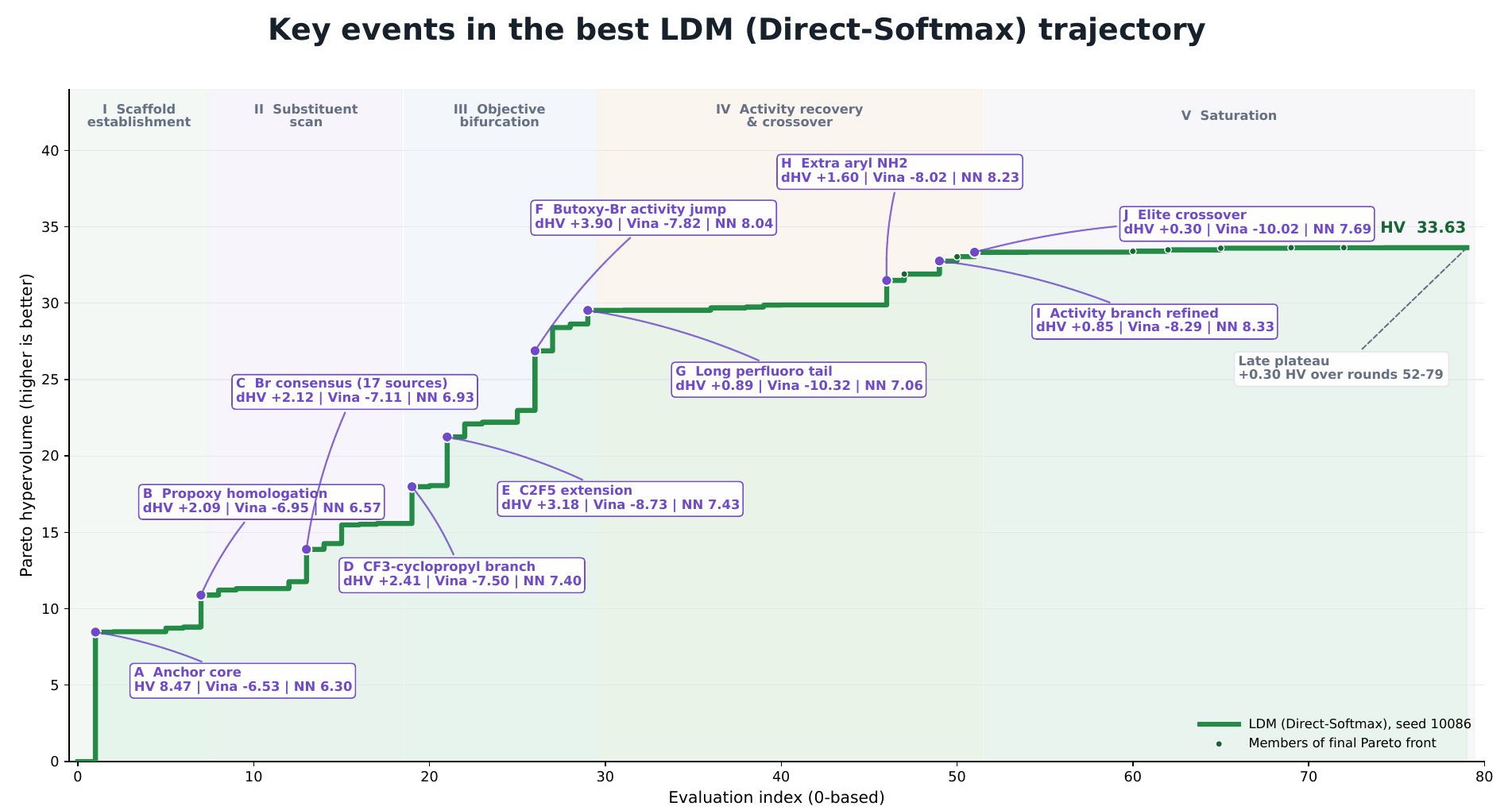
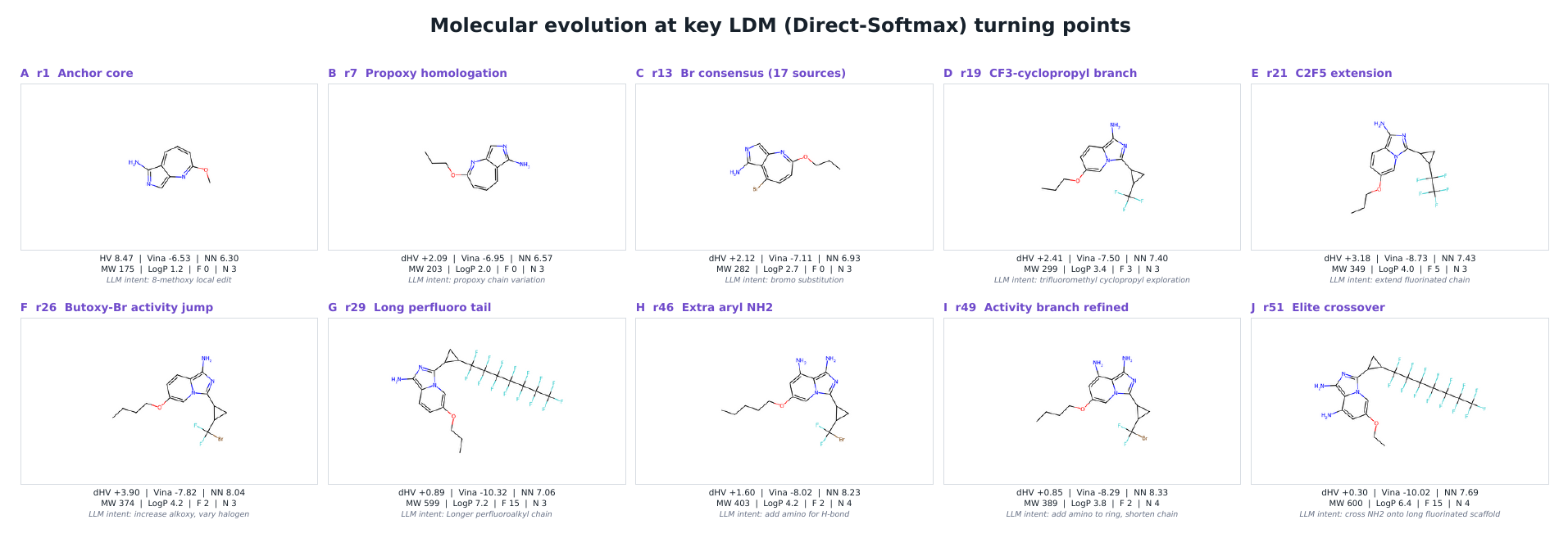
Why the score keeps rising: jumps in the curve correspond to five interpretable stages: establishing scaffolds, scanning substituents, branching by objective, recombining across families, and only then reaching saturation.The changes are not merely local edits to one molecule: ten milestones show the system switching scaffolds and functional-group combinations, changing the searchable structural space itself.
IMPORTANT NOTEThese results show that LDM found stronger candidates under the paper’s computational evaluation metrics. They do not establish that an antibody binds in the laboratory or that a molecule is effective, safe or possible to synthesise. Those candidates still require higher-fidelity modelling and wet-lab validation.
This page focuses on the main results. Full experimental settings, baselines, statistical reporting and ablations are in Section 6 and the appendices of the paper.
FROM SEARCH TO A LEARNED STRATEGY
Do not just remember the winner. Learn why it was worth trying.
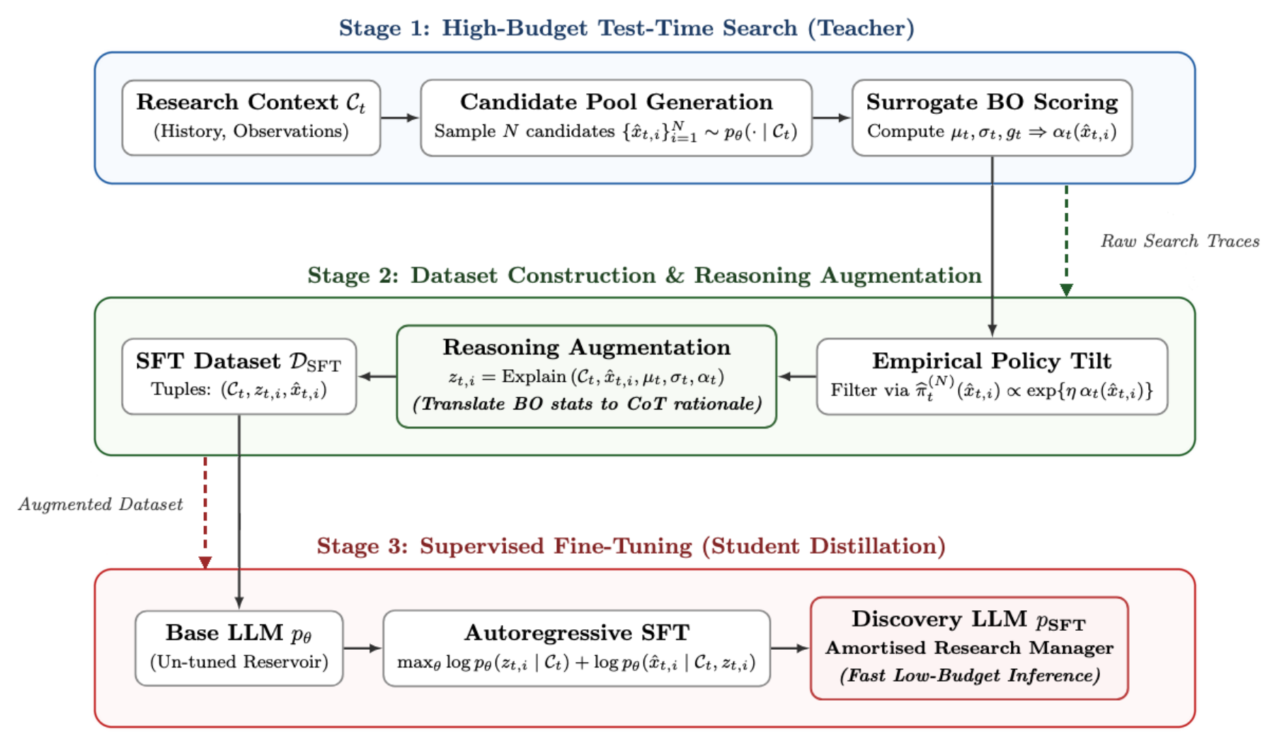
High-budget search produces more than candidates. It creates a trajectory of where the research stands, why a candidate was chosen, and which barrier should be crossed next. LDM distils this discovery strategy into a smaller model.
Search trajectories are translated into “action + rationale,” then used to train a lighter-weight proposal model.
KRAS G12D26.660±2.608
fine-tuned + research rationale
SAME STUDENT22.279±3.828
fine-tuned, no research rationale
BASE MODEL16.489±5.867
base model without fine-tuning
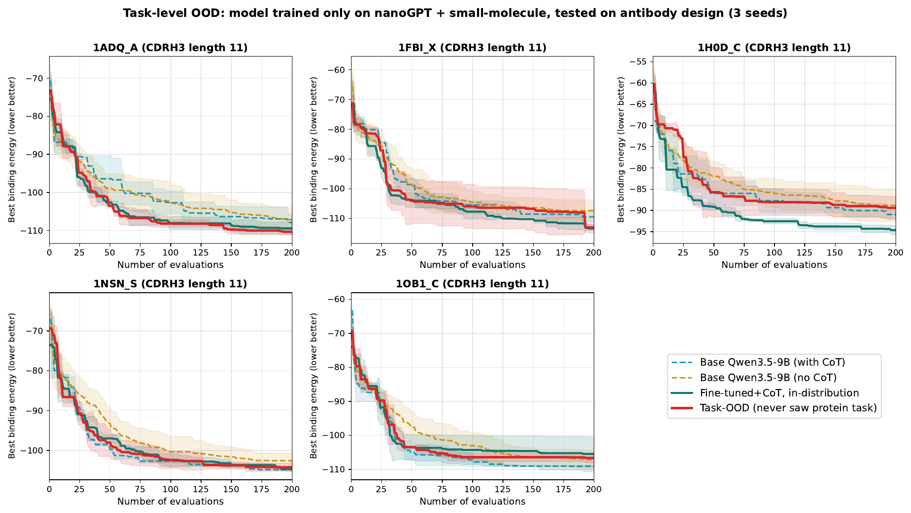
What transfers and what does not: a model trained only on nanoGPT and small-molecule trajectories, with no protein data, matches or exceeds the in-distribution antibody model on four of five targets. The exception, 1H0D_C, requires de novo motif design rather than candidate selection alone.
What a search trajectory contains
Candidates, surrogate scores, constraints, failure records, whether the search has stalled, and the research state: exploit, explore, or open a new dimension next.
What the rationale explains
It does not explain why the final answer is good. It explains why, given the current evidence, this candidate deserves one scarce evaluation now.
What transfer suggests
The new task-level test removes antibodies from training entirely. Matching the in-distribution model on four of five antigens shows that acquisition-guided research strategy transfers across domains; the 1H0D_C failure isolates what does not transfer: protein-specific de novo design.
The purpose of distillation is to turn “why this next step is worth taking” into a model capability.In AutoResearch, the fine-tuned Qwen3.5-9B with research rationales reaches 0.9788, outperforming the paper’s Qwen3-Coder-30B reference value of 0.9801. The comparable fine-tuned model without rationale augmentation reaches 0.9829.
These are reported reference results, not a size-matched, same-backbone comparison.